
One of the biggest challenges in real-world machine learning is that supervised models require labeled data—yet in many practical scenarios, the data you start with is almost always unlabeled. Manually annotating thousands of samples isn’t just slow; it’s expensive, tedious, and often impractical.
This is where active learning becomes a game-changer.
Active learning is a subset of machine learning in which the algorithm is not a passive consumer of data—it becomes an active participant. Instead of labeling the entire dataset upfront, the model intelligently selects which data points it wants labeled next. It interactively queries a human or oracle for labels on the most informative samples, allowing it to learn faster using far fewer annotations. Check out the FULL CODES here.
Here’s how the workflow typically looks:

- Begin by labeling a small seed portion of the dataset to train an initial, weak model.
- Use this model to generate predictions and confidence scores on the unlabeled data.
- Compute a confidence metric (e.g., probability gap) for each prediction.
- Select only the lowest-confidence samples—the ones the model is most unsure about.
- Manually label these uncertain samples and add them to the training set.
- Retrain the model and repeat the cycle of predict → rank confidence → label → retrain.
- After several iterations, the model can achieve near–fully supervised performance while requiring far fewer manually labeled samples.
In this article, we’ll walk through how to apply this strategy step-by-step and show how active learning can help you build high-quality supervised models with minimal labeling effort. Check out the FULL CODES here.
Installing & Importing the libraries
import numpy as np
import matplotlib.pyplot as plt
from sklearn.datasets import make_classification
from sklearn.linear_model import LogisticRegression
from sklearn.model_selection import train_test_split
from sklearn.metrics import accuracy_score
For this tutorial, we will be using the make_classification dataset from the sklearn library
N_SAMPLES = 1000 # Total number of data points
INITIAL_LABELED_PERCENTAGE = 0.10 # Your constraint: Start with 10% labeled data
NUM_QUERIES = 20 # Number of times we ask the “human” to label a confusing sample
NUM_QUERIES = 20 represents the annotation budget in an active learning setup. In a real-world workflow, this would mean the model selects the 20 most confusing samples and sends them to human annotators to label—each annotation costing time and money. In our simulation, we replicate this process automatically: during each iteration, the model selects one uncertain sample, the code instantly retrieves its true label (acting as the human oracle), and the model is retrained with this new information.
Thus, setting NUM_QUERIES = 20 means we’re simulating the benefit of labeling only 20 strategically chosen samples and observing how much the model improves with that limited but valuable human effort.
Data Generation and Splitting Strategy for Active Learning
This block handles data generation and the initial split that powers the entire Active Learning experiment. It first uses make_classification to create 1,000 synthetic samples for a two-class problem. The dataset is then split into a 10% held-out test set for final evaluation and a 90% pool for training. From this pool, only 10% is kept as the small initial labeled set—matching the constraint of starting with very limited annotations—while the remaining 90% becomes the unlabeled pool. This setup creates the realistic low-label scenario Active Learning is designed for, with a large pool of unlabeled samples ready for strategic querying. Check out the FULL CODES here.
n_samples=N_SAMPLES, n_features=10, n_informative=5, n_redundant=0,
n_classes=2, n_clusters_per_class=1, flip_y=0.1, random_state=SEED
)
# 1. Split into 90% Pool (samples to be queried) and 10% Test (final evaluation)
X_pool, X_test, y_pool, y_test = train_test_split(
X, y, test_size=0.10, random_state=SEED, stratify=y
)
# 2. Split the 90% Pool into Initial Labeled (10% of the pool) and Unlabeled (90% of the pool)
X_labeled_current, X_unlabeled_full, y_labeled_current, y_unlabeled_full = train_test_split(
X_pool, y_pool, test_size=1.0 – INITIAL_LABELED_PERCENTAGE,
random_state=SEED, stratify=y_pool
)
# A set to track indices in the unlabeled pool for efficient querying and removal
unlabeled_indices_set = set(range(X_unlabeled_full.shape[0]))
print(f”Initial Labeled Samples (STARTING N): {len(y_labeled_current)}”)
print(f”Unlabeled Pool Samples: {len(unlabeled_indices_set)}”)
Initial Training and Baseline Evaluation
This block trains the initial Logistic Regression model using only the small labeled seed set and evaluates its accuracy on the held-out test set. The labeled sample count and baseline accuracy are then stored as the first points in the performance history, establishing a starting benchmark before Active Learning begins. Check out the FULL CODES here.
accuracy_history = []
# Train the baseline model on the small initial labeled set
baseline_model = LogisticRegression(random_state=SEED, max_iter=2000)
baseline_model.fit(X_labeled_current, y_labeled_current)
# Evaluate performance on the held-out test set
y_pred_init = baseline_model.predict(X_test)
accuracy_init = accuracy_score(y_test, y_pred_init)
# Record the baseline point (x=90, y=0.8800)
labeled_size_history.append(len(y_labeled_current))
accuracy_history.append(accuracy_init)
print(f”INITIAL BASELINE (N={labeled_size_history[0]}): Test Accuracy: {accuracy_history[0]:.4f}”)
Active Learning Loop
This block contains the heart of the Active Learning process, where the model iteratively selects the most uncertain sample, receives its true label, retrains, and evaluates performance. In each iteration, the current model predicts probabilities for all unlabeled samples, identifies the one with the highest uncertainty (least confidence), and “queries” its true label—simulating a human annotator. The newly labeled data point is added to the training set, a fresh model is retrained, and accuracy is recorded. Repeating this cycle for 20 queries demonstrates how targeted labeling quickly improves model performance with minimal annotation effort. Check out the FULL CODES here.
print(f”\nStarting Active Learning Loop ({NUM_QUERIES} Queries)…”)
# ———————————————–
# The Active Learning Loop (Query, Annotate, Retrain, Evaluate)
# Purpose: Run 20 iterations to demonstrate strategic labeling gains.
# ———————————————–
for i in range(NUM_QUERIES):
if not unlabeled_indices_set:
print(“Unlabeled pool is empty. Stopping.”)
break
# — A. QUERY STRATEGY: Find the Least Confident Sample —
# 1. Get probability predictions from the CURRENT model for all unlabeled samples
probabilities = current_model.predict_proba(X_unlabeled_full)
max_probabilities = np.max(probabilities, axis=1)
# 2. Calculate Uncertainty Score (1 – Max Confidence)
uncertainty_scores = 1 – max_probabilities
# 3. Identify the index of the sample with the MAXIMUM uncertainty score
current_indices_list = list(unlabeled_indices_set)
current_uncertainty = uncertainty_scores[current_indices_list]
most_uncertain_idx_in_subset = np.argmax(current_uncertainty)
query_index_full = current_indices_list[most_uncertain_idx_in_subset]
query_uncertainty_score = uncertainty_scores[query_index_full]
# — B. HUMAN ANNOTATION SIMULATION —
# This is the single critical step where the human annotator intervenes.
# We look up the true label (y_unlabeled_full) for the sample the model asked for.
X_query = X_unlabeled_full[query_index_full].reshape(1, -1)
y_query = np.array([y_unlabeled_full[query_index_full]])
# Update the Labeled Set: Add the new annotated sample (N becomes N+1)
X_labeled_current = np.vstack([X_labeled_current, X_query])
y_labeled_current = np.hstack([y_labeled_current, y_query])
# Remove the sample from the unlabeled pool
unlabeled_indices_set.remove(query_index_full)
# — C. RETRAIN and EVALUATE —
# Train the NEW model on the larger, improved labeled set
current_model = LogisticRegression(random_state=SEED, max_iter=2000)
current_model.fit(X_labeled_current, y_labeled_current)
# Evaluate the new model on the held-out test set
y_pred = current_model.predict(X_test)
accuracy = accuracy_score(y_test, y_pred)
# Record results for plotting
labeled_size_history.append(len(y_labeled_current))
accuracy_history.append(accuracy)
# Output status
print(f”\nQUERY {i+1}: Labeled Samples: {len(y_labeled_current)}”)
print(f” > Test Accuracy: {accuracy:.4f}”)
print(f” > Uncertainty Score: {query_uncertainty_score:.4f}”)
final_accuracy = accuracy_history[-1]
Final Result
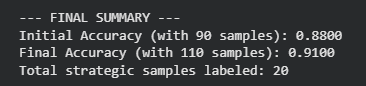
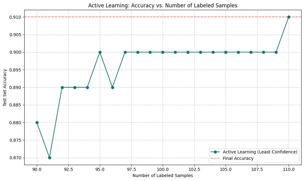
The experiment successfully validated the efficiency of Active Learning. By focusing annotation efforts on only 20 strategically selected samples (increasing the labeled set from 90 to 110), the model’s performance on the unseen Test Set improved from 0.8800 (88%) to 0.9100 (91%).
This 3 percentage point increase in accuracy was achieved with a minimal increase in annotation effort—roughly a 22% increase in the size of the training data resulted in a measurable and meaningful performance boost.
In essence, the Active Learner acts as an intelligent curator, ensuring that every dollar or minute spent on human labeling provides the maximum possible benefit, proving that smart labeling is far more valuable than random or bulk labeling. Check out the FULL CODES here.
Plotting the results
plt.plot(labeled_size_history, accuracy_history, marker=”o”, linestyle=”-“, color=”#00796b”, label=”Active Learning (Least Confidence)”)
plt.axhline(y=final_accuracy, color=”red”, linestyle=”–“, alpha=0.5, label=”Final Accuracy”)
plt.title(‘Active Learning: Accuracy vs. Number of Labeled Samples’)
plt.xlabel(‘Number of Labeled Samples’)
plt.ylabel(‘Test Set Accuracy’)
plt.grid(True, linestyle=”–“, alpha=0.7)
plt.legend()
plt.tight_layout()
plt.show()
Check out the FULL CODES here. Feel free to check out our GitHub Page for Tutorials, Codes and Notebooks. Also, feel free to follow us on Twitter and don’t forget to join our 100k+ ML SubReddit and Subscribe to our Newsletter. Wait! are you on telegram? now you can join us on telegram as well.

I am a Civil Engineering Graduate (2022) from Jamia Millia Islamia, New Delhi, and I have a keen interest in Data Science, especially Neural Networks and their application in various areas.